4  Taxonomic Analysis

Following taxonomic classification and exploratory visualization, downstream analyses were conducted in R to characterize microbial groups associated with Deroceras laeve.

This chapter presents an example workflow using Archaea as a representative taxonomic subset. The same strategy can be applied to Bacteria, Fungi, Viruses, or other groups of interest by modifying the selected taxonomic level.

Input Data

Kraken2-derived BIOM files were imported into R using the phyloseq package.

Code

library(phyloseq)
library(ggplot2)
library(dplyr)

dlaeve_physeq <- import_biom("dlaeve_taxonomy.biom")

Taxonomic labels were curated by removing unnecessary prefixes and assigning standardized rank names.

Code

dlaeve_physeq@tax_table@.Data <-
  substring(dlaeve_physeq@tax_table@.Data, 4)

colnames(dlaeve_physeq@tax_table@.Data) <- c(
  "Kingdom", "Phylum", "Class",
  "Order", "Family", "Genus", "Species"
)

4.1 Example Workflow: Archaea

Taxonomic Selection

Reads assigned to Archaea were extracted for focused downstream analyses.

Code

archaea <- subset_taxa(
  dlaeve_physeq,
  Kingdom == "Archaea"
)

4.1.1 Removal of Unidentified Genera

Only classified genera were retained for abundance summaries and visualization.

Code

archaea <- subset_taxa(
  archaea,
  Genus != ""
)

4.1.2 Relative Abundance Transformation

Code

percentages <- transform_sample_counts(
  archaea,
  function(x) x * 100 / sum(x)
)

4.2 Phylum-Level Summarization

Code

percentages_glom <- tax_glom(
  percentages,
  taxrank = "Phylum"
)

percentages_df <- psmelt(
  percentages_glom
)

4.2.1 Identification of Dominant Taxa

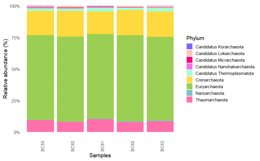
The ten most abundant phyla were selected, while less abundant taxa were grouped as Others.

Code

abundance_phylum <- percentages_df %>%
  mutate(Phylum = as.character(Phylum)) %>%
  group_by(Phylum) %>%
  summarize(Abundance = mean(Abundance)) %>%
  arrange(desc(Abundance)) %>%
  slice_head(n = 10)

4.2.2 Visualization

Relative abundance plots were generated with ggplot2 using custom color palettes.

Custom colors:

Code

colors <- c(
  "#9BCF53", "#FFD93D", "#FF70AB",
  "#A3FFD6", "#FEC7B4", "#83C0C1",
  "#FF0080", "#F273E6", "#7B66FF",
  "#FFF67E"
)

colors_by_phylum <- setNames(
  colors[1:nrow(abundance_phylum)],
  abundance_phylum$Phylum
)

colors_by_phylum["Others"] <- "#A7BED3"

Plot:

Code

ggplot(
  percentages_df,
  aes(
    x = Sample,
    y = Abundance,
    fill = Phylum
  )
) +
  geom_bar(
    stat = "identity",
    position = "fill"
  ) +
  scale_fill_manual(values = colors_by_phylum) + 
  theme_minimal(base_size = 14) +
  theme(
    axis.text.x = element_text(
      angle = 90,
      hjust = 1
    )
  ) +
  scale_y_continuous(
    labels = scales::percent_format()
  ) +
  labs(
    x = "Samples",
    y = "Relative abundance (%)"
  )

4.3 Genus-Level Analysis

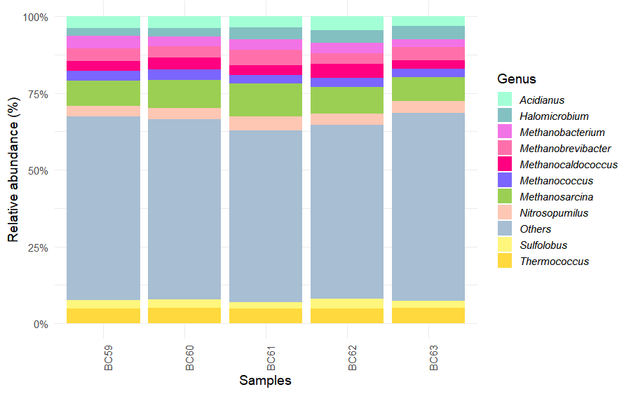
To further refine the archaeal community profile, reads were also summarized at the genus level.

Code

genus_glom <- tax_glom(
  percentages,
  taxrank = "Genus"
)

genus_df <- psmelt(
  genus_glom
)

4.3.1 Identification of Dominant Genera

The ten most abundant genera were selected, while less abundant taxa were grouped as Others.

Code

abundance_genus <- genus_df %>%
  mutate(
    Genus = as.character(Genus)
  ) %>%
  group_by(Genus) %>%
  summarize(
    Abundance = mean(Abundance),
    .groups = "drop"
  ) %>%
  arrange(desc(Abundance)) %>%
  slice_head(n = 10)

genus_df <- genus_df %>%
  mutate(
    Genus = ifelse(
      Genus %in% abundance_genus$Genus,
      Genus,
      "Others"
    )
  )

4.3.2 Visualization

Relative abundance plots were generated using the same custom palette employed for phylum-level summaries.

Code

colors_by_genus <- setNames(
  colors[1:nrow(abundance_genus)],
  abundance_genus$Genus
)

colors_by_genus["Others"] <- "#A7BED3"

ggplot(
  genus_df,
  aes(
    x = Sample,
    y = Abundance,
    fill = Genus
  )
) +
  geom_bar(
    stat = "identity",
    position = "fill"
  ) +
  scale_fill_manual(
    values = colors_by_genus
  ) +
  theme_minimal(base_size = 14) +
  theme(
    axis.text.x = element_text(
      angle = 90,
      hjust = 1
    ),
    legend.text = element_text(
      face = "italic"
    )
  ) +
  scale_y_continuous(
    labels = scales::percent_format()
  ) +
  labs(
    x = "Samples",
    y = "Relative abundance (%)"
  )

4.4 Adaptation to Other Taxa

The same analytical framework can be applied to other microbial groups by modifying the selected taxonomic subset according to the rank of interest and the structure of the dataset.

For example, some groups can be selected directly at the Kingdom level:

Code

subset_taxa(dlaeve_physeq, Kingdom == "Bacteria")
subset_taxa(dlaeve_physeq, Kingdom == "Viruses")

In other cases, more specific taxonomic ranks may be used. For fungal analyses, representative phyla were selected as follows:

Code

subset_taxa( dlaeve_physeq, 
             Phylum %in% c("Ascomycota", "Basidiomycota", "Microsporidia" )
  )